
Softmax Transformation
When I train my neural network models, I often use the method called “Softmax Transformation”. It is the method of representing the training data into the sparse form. When I first learned how to do it, I had some troubles ‘cause there wasn’t enough example about how to do it. And still, I can’t find nice explanation about the softmax transformation with examples. So here I have some brief explanation and sample codes for the softmax transformation. Let’s see how the softmax transformation works step by step.
Basic Idea
Basically, you can consider it as the sparse representation of the data. Then, why do we need it? It has been known that the sparse encoding eases the difficulty of training.
Let’s assume that the training data for the recurrent neural network model is the trajectory of the robot’s joints. If we want to train the model to generate 1-step look-ahead prediction, we might need the training data in the form of 2 column x N lines, where N is the length of the data.
Of course, we can train the network with those values. However, learning will be much easier if those values are represented in the sparse form and given to the model (we’ll see why later).
So here is an example. Let’s say the softmax dimension is 10. It means that one value (e.g., elbow’s position value which range from -90 to 90) will be represented with 10 softmax values (which range from 0 to 1). That is, after the softmax transformation, the single value (hereafter, analog value) is converted into a set of values (hereafter, softmax values). For example, the analog value 34 can be represented by something like {0.0, 0.0, 0.3, 0.5, 0.2, 0.0, 0.0, 0.0, 0.0, 0.0}. Note that the sum of the softmax values is constrained to be 1.
Note that the softmax transformation in this article is slightly different from softmax function or softmax activation function. According to Wikipedia, the softmax function is
a generalization of the logistic function that “squashes” a K-dimensional vector z of arbitrary real values to a K-dimensional vector σ(z) of real values in the range [0, 1] that add up to 1.
The Matlab code and the sample data used in this tutorial can be downloaded from here.
Softmax transformation - How Do We Do It
Throughout the examples, I’ll assume the followings:
- 2 analog values - It means the training data has 2 dimensional values, such as two joint angles (e.g., left & right elbows). I’ll assume that the ranges of those two values are same (-2.5 to 2.5). Of course, each analog value can have different ranges depending on the experiments. Even if that’s the case, the basic idea is same. It wouldn’t change a code a lot, just a bit more complicated. That’s all.
- 10 softmax dimensions - This means that one single analog value will be represented as 10 dimensional softmax values ranging from 0 to 1. In general, more softmax dimension brings the better results and I’ve found that 10 softmax dimensions worked quite well in many of my past experiments.
- Since we assume 2 analog values and 10 softmax dimensions, there will be 2 x 10 neurons at the input/output layers of the neural network model.
So let’s see the equation first.
softmax refers the softmax transformed value which has 10 dimensions (J = softmax dimension). analog is the 1-dimensional analog value that needs to be transformed. ref is the reference points which consists of the J values (in this case, 10). This is obtained by sampling J values from MIN and MAX where MIN & MAX denote the minimum and maximum of the analog value. It can be computed in Matlab easily by using references = linspace(minVal,maxVal,softmaxUnit). Note that if the each analog value has the different range, then the different ref should be used in computation. sigma is a value that specifies the shape of the distribution. You’ll see the effect of sigma on softmax transformation later in this tutorial.
Let’s start with the example Matlab code. If you open the data_analog.txt looks like this:
|
|
Each column corresponds to the analog value (e.g., joint angle) and each row corresponds to the time step (1000 steps in the example).
So, the first thing you do is setting the softmax transformation parameters.
|
|
softmaxUnit refers the number of softmax units per analog dimension (J in the equation). In this tutorial, it is 10. minVal and maxVal refer the range of the analog value. I assumed that they have same range (-2.5 to 2.5). But as you can see in the code, I added a bit of margin and I set the minimum and the maximum as -3 and 3 respectively to ensure that the values near the extremes can be also transformed well. SIGMA is a value that specifies the shape of the distribution. You’ll see the effect of SIGMA on softmax transformation later in this tutorial.
Now, let’s transformation the analog values to the softmax representation.
|
|
The code is quite straightforward. The code first computes the reference points: references = linspace(minVal,maxVal,softmaxUnit);
Then, it computes the value of each softmax value (val(1,idxRef)) as specified in the equation. So 1-dimensional analog value (traj(idxStep,idxJnt)) is converted to 10-dimensional softmax values (val).
After the transformation, you will have the softmax representation file (data_softmax.txt) which looks like this:
|
|
Each row has 20 columns (2 analog dimension x 10 softmax dimension) and it has 1000 rows (steps). At each row, the first 10 values are the softmax values for the first analog value.
Inverse Softmax transformation - Why & How Do We Do It
Ok, you can train the network with the softmax transformed values. Then, why do we need the inverse transformation? It’s because we (usually) want to check the model’s output on a robot (or at least we want to plot it). It’d be much easier to check the result with analog form rather than the softmax form.
So let’s see how we convert the softmax values back to the analog values. The equations is as follows:
and the inverse softmax transformation is conducted as follows:
|
|
The code reads each 10 columns (softmax(idxJnt:idxJnt+softmaxUnit-1)) and multiplies it with the references (transposed). After this computation, there will be 1 analog value. After the inverse transform, there will be data_analog_inverse.txt which looks like this:
|
|
This is the analog value obtained from the softmax values. If the transform was successful, there shouldn’t be huge differences between the original and the inverted values. So.. let’s check it.
Check the Transformation Result
Whenever you transformation the analog values to softmax representation, it’s always a good idea to check the transformed result. To check the transformation performance, I’ll compare the original analog value (data_analog.txt) with the inversely transformed value (data_analog_inverse.txt). This is how I do it.
|
|
Once you run this code, you will have 2 plots. The one on the left is the trajectories of the original analog values (solid lines) and the inversely transformed analog values (dashed lines). If the solid and the dashed lines are completely overlapped, it means the transformation was successful.
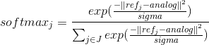
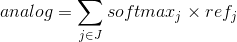
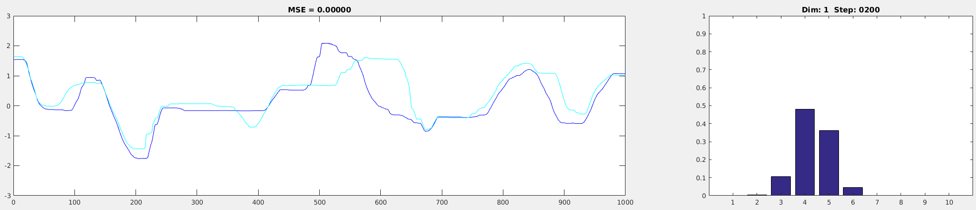
The performance of the softmax transformation relies on 2 things: SIGMA and the range of the analog value (minVal, maxVal). And belows are the example of the output with the different SIGMA value.
sigma = 0.01:
 sigma = 0.01
sigma = 0.1:
 sigma = 0.1
sigma = 0.5:
 sigma = 0.5
As you can see from the pictures above, the transformation performance is the best when SIGMA is set to 0.5. In addition, you can see that the softmax values are nicely distributed along the several dimensions (the right figure). By having a such distribution, there’d be more overlapped parts in two adjacent data, making training easier. If it has a peaky distribution (e.g., SIGMA = 0.01), there’d be less (or no) overlap between the consecutive data, making training harder.
Also, check the transformation performance of the values near the extremes (minimum and maximum values in the analog data). Based on the setting (minVal, maxVal), it might not be transformed well. So make sure the whole trajectory was transformed well before proceeding to training (In this case, everything looks okay).
Final Remarks - DOs & DON’Ts
Do
- If the analog values have different ranges, do set the different ranges during the softmax transformation. It’ll generally bring the better results.
- Checked the transformed results of the extreme values (minimum and maximum). If the extreme values are not transformed well, adjust the margin in the range of the analog value.
Don’t
- You don’t want to have a peaky distribution. Choose the appropriate sigma value.
The Complete Matlab Code and the Sample Data
Here is the Matlab code and the sample data. Download
References
- Softmax Function Wikipedia
- Hwang, J., & Tani, J. (2017). Seamless Integration and Coordination of Cognitive Skills in Humanoid Robots: A Deep Learning Approach. IEEE Transactions on Cognitive and Developmental Systems (TCDS). arXiv
- Hwang, J., Kim, J., Ahmadi, A., Choi, M., & Tani, J. (2017). Predictive Coding-based Deep Dynamic Neural Network for Visuomotor Learning. In 2017 Joint IEEE International Conference on Development and Learning and Epigenetic Robotics (ICDL-EpiRob) arXiv
